在最新版本的Excel里面,更新了很多新函数,其中TOCOL函数公式非常强大,值得一学,从字面意义可以理解出来,它是将数据转换成一列的
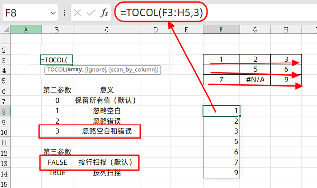
1、基本用法当我们在单元格中输入公式,它是由三个参数组成的
=TOCOL(数组区域,第二参数,第三参数)
第二参数和第三参数,是固定的填写数字,对应的意义如下所示:

所以,当我们输入公式:
=TOCOL(F3:H5,3)
它会对F3:H5中间的数据区域,忽略空白和错误值,按行扫描,堆积成一列数据,得到的结果如下所示:
如果我们使用的公式是:
=TOCOL(F3:H5,0,TRUE)
它会保留所有的值,按列扫描的排列,空白单元格会被自动填充数字0
 2、组合用法:TOCOL+UNQIUE
我们想提取A:C列中的不重复数据名单
可以使用公式:
=UNIQUE(TOCOL(A:C,1))
TOCOL,第2参数为1表示忽略空白单元格,排成一列,再用UNQUE函数公式可以去一次重,得到唯一的数据列
 3、指定次数重复数据
我们想根据指定的次数来重复数据,得到对应的结果

我们只需要使用公式:
=TOCOL(IF(B2:B4>=COLUMN($1:$1000),A2:A4,NA()),2)
一次性的得到所有的结果
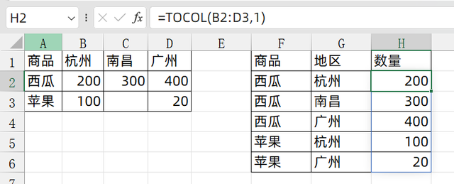
 4、数据逆透视
我们希望从左边的数据区域,转换成右边的数据区域
通常我们用PQ的逆透视来完成,但是其实也可以用TOCOL公式来完成

当我们输入公式:
=TOCOL(IF(B2:D3<>"",A2:A3,NA()),2)
可以将商品字段下面的数据全部填充出来

然后地区数据,使用公式:
=TOCOL(IF(B2:D3<>"",B1:D1,NA()),2)

数量字段使用的公式是:
=TOCOL(B2:D3,1)
关于这个函数公式,你学会了么?动手试试吧!
