生成式大语言模型(LLM)可以针对各种用户的 prompt 生成高度流畅的回复。然而,大模型倾向于产生幻觉或做出非事实陈述,这可能会损害用户的信任。
大语言模型的长而详细的输出看起来很有说服力,但是这些输出很有可能是虚构的。这是否意味着我们不能信任聊天机器人,每次都必须手动检查输出的事实?有一些方法可以让聊天机器人在适当的保护措施下不太可能说假话。
一个最简单的方法就是调整temperature到一个很大的值,例如0.7,然后使用相同的提问多次对话。这样得到的输出应该只会改变句子的结构,输出之间的差异应该只是语义上的,而不是事实上的。

这个简单的想法允许引入一种新的基于样本的幻觉检测机制。如果LLM对同一提示的输出相互矛盾,它们很可能是幻觉。如果它们相互关联,就意味着信息是真实的。对于这种类型的求值,我们只需要llm的文本输出。这被称为黑盒评估。
余弦距离余弦距离(Cosine Distance)是衡量两个向量之间相似度的一种度量方法,通常用于文本相似性、推荐系统和机器学习等领域。我们可以计算嵌入句子的对应对之间的两两余弦相似度。下面的函数将最初生成的句子output和一个包含3个示例输出的列表sampled_passages作为输入。
这里使用了all-MiniLM-L6-v2轻量模型。嵌入一个句子会把它变成它的向量表示。
output = "Evelyn Hartwell is a Canadian dancer, actor, and choreographer." output_embeddings= model.encode(output)array([ 6.09108340e-03, -8.73148292e-02, -5.30637987e-02, -4.41815751e-03, 1.45469820e-02, 4.20340300e-02, 1.99541822e-02, -7.29453489e-02,… -4.08893749e-02, -5.41420840e-02, 2.05906332e-02, 9.94611382e-02, -2.24501686e-03, 2.29083393e-02, 7.80007839e-02, -9.53456461e-02], dtype=float32)
将LLM的每个输出生成嵌入,然后使用sentence_transformers中的pairwise_cos_sim函数计算cos相似度。将原始响应与每个新样本响应进行比较,然后求平均值。
from sentence_transformers.util import pairwise_cos_simfrom sentence_transformers import SentenceTransformerdef get_cos_sim(output,sampled_passages): model = SentenceTransformer('all-MiniLM-L6-v2') sentence_embeddings = model.encode(output).reshape(1, -1) sample1_embeddings = model.encode(sampled_passages[0]).reshape(1, -1) sample2_embeddings = model.encode(sampled_passages[1]).reshape(1, -1) sample3_embeddings = model.encode(sampled_passages[2]).reshape(1, -1) cos_sim_with_sample1 = pairwise_cos_sim( sentence_embeddings, sample1_embeddings ) cos_sim_with_sample2 = pairwise_cos_sim( sentence_embeddings, sample2_embeddings ) cos_sim_with_sample3 = pairwise_cos_sim( sentence_embeddings, sample3_embeddings ) cos_sim_mean = (cos_sim_with_sample1 + cos_sim_with_sample2 + cos_sim_with_sample3) / 3 cos_sim_mean = cos_sim_mean.item() return round(cos_sim_mean,2)

从上面的图像可以看到矢量之间的角度大约是30⁰,因此它们彼此接近。余弦大约是0.87。余弦函数越接近1,这两个向量就越接近。
cos_sim_score = get_cos_sim(output, [sample1,sample2,sample3])
嵌入的cos_sim_score的平均值为0.52。
为了理解如何解释这个数字,让我们将其与一些有效输出的余弦相似度评分进行比较

这个输出的余弦相似度为0.93。所以说第一个输出很有可能是LLM的幻觉。
BERTScoreBERTScore建立在两两余弦相似度思想的基础上。

用于计算上下文嵌入的标记器是RobertaTokenizer。上下文嵌入不同于静态嵌入,因为它们会考虑单词周围的上下文。
def get_bertscore(output, sampled_passages): # spacy sentence tokenization sentences = [sent.text.strip() for sent in nlp(output).sents] selfcheck_bertscore = SelfCheckBERTScore(rescale_with_baseline=True) sent_scores_bertscore = selfcheck_bertscore.predict( sentences = sentences, # list of sentences sampled_passages = sampled_passages, # list of sampled passages ) df = pd.DataFrame({ 'Sentence Number': range(1, len(sent_scores_bertscore) + 1), 'Hallucination Score': sent_scores_bertscore }) return df
selfcheck_bertscore没有将完整的原始输出作为参数传递,而是将其分成单独的句子。
['Evelyn Hartwell is an American author, speaker, and life coach.', 'She is best known for her book, The Miracle of You: How to Live an Extraordinary Life, which was published in 2007.', 'She is a motivational speaker and has been featured on TV, radio, and in many magazines.', 'She has authored several books, including How to Make an Impact and The Power of Choice.']
这一步很重要,因为selfcheck_bertscore.predict函数将每个句子的BERTScore计算为与样本中每个句子匹配的原始响应。它创建一个数组,其行数等于原始输出中的句子数,列数等于样本数。
array([[0., 0., 0.], [0., 0., 0.], [0., 0., 0.], [0., 0., 0.]])
用于计算候选句子和参考句子之间BERTScore的模型是RoBERTa large,共17层。最初的输出有4个句子,分别是r1 r2 r3和r4。第一个样本有两个句子:c1和c2。计算原始输出中的每个句子与第一个样本中的每个句子匹配的F1 BERTScore。然后我们对基线张量b =([0.8315,0.8315,0.8312])进行缩放。基线b是使用来自Common Crawl单语数据集的100万个随机配对句子来计算的。他们计算了每一对的BERTScore,并取其平均值。这代表了一个下界,因为随机对几乎没有语义重叠。

保留原始回复中每个句子的BERTScore,并从每个抽取的样本中选择最相似的句子。其逻辑是,如果一条信息出现在由同一提示生成的多个样本中,那么该信息很有可能是真实的。如果一个语句只出现在一个示例中,而没有出现在来自同一提示的任何其他示例中,则更有可能是伪造的。
所以我们计算最大相似度:
bertscore_arrayarray([[0.43343216, 0. , 0. ], [0.12838356, 0. , 0. ], [0.2571277 , 0. , 0. ], [0.21805632, 0. , 0. ]])
对另外两个样本重复这个过程:
array([[0.43343216, 0.34562832, 0.65371764], [0.12838356, 0.28202596, 0.2576825 ], [0.2571277 , 0.48610589, 0.2253703 ], [0.21805632, 0.34698656, 0.28309497]])
然后我们计算每行的平均值,给出原始回复中每个句子与每个后续样本之间的相似度得分。
array([0.47759271, 0.22269734, 0.32286796, 0.28271262])
每句话的幻觉得分是通过从上面的每个值中减去1得到的。

将结果与尼古拉斯·凯奇(Nicolas Cage)的答案进行比较。
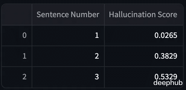
有效输出的幻觉得分较低,而虚构输出的幻觉得分较高。但是计算BERTScore的过程非常耗时,这使得它不适合用于实时幻觉检测。
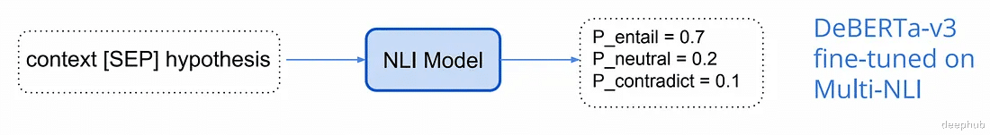
NLI自然语言推理(NLI)涉及确定一个假设在逻辑上是遵循给定前提还是与给定前提相矛盾。这种关系可分为牵连、矛盾或中立。对于NLI,我们利用在MNLI数据集上进行微调的DeBERTa-v3-large模型来执行NLI。
下面是一些前提-假设对及其标签的例子。

def get_self_check_nli(output, sampled_passages): # spacy sentence tokenization sentences = [sent.text.strip() for sent in nlp(output).sents] selfcheck_nli = SelfCheckNLI(device=mps_device) # set device to 'cuda' if GPU is available sent_scores_nli = selfcheck_nli.predict( sentences = sentences, # list of sentences sampled_passages = sampled_passages, # list of sampled passages ) df = pd.DataFrame({ 'Sentence Number': range(1, len(sent_scores_nli) + 1), 'Probability of Contradiction': sent_scores_nli }) return df
在selfcheck_nli.predict函数,原始响应中的每个句子都与三个样本中的每个配对。
logits = model(**inputs).logits # neutral is already removedprobs = torch.softmax(logits, dim=-1)prob_ = probs[0][1].item() # prob(contradiction)

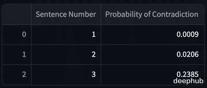
现在我们对这四个句子中的每一个重复这个过程。

可以看到,模型输出的矛盾概率非常高。现在我们将其与实际输出进行比较。
这个模特做得很好!但是NLI检查时间有点太长了。

较新的方法已经开始使用llm本身来评估生成的文本。而不是使用公式来计算分数,我们将输出与三个样本一起发送到gpt-3.5 turbo。该模型将决定原始输出相对于生成的其他三个样本的一致性。
def llm_evaluate(sentences,sampled_passages): prompt = f"""You will be provided with a text passage \ and your task is to rate the consistency of that text to \ that of the provided context. Your answer must be only \ a number between 0.0 and 1.0 rounded to the nearest two \ decimal places where 0.0 represents no consistency and \ 1.0 represents perfect consistency and similarity. \n\n \ Text passage: {sentences}. \n\n \ Context: {sampled_passages[0]} \n\n \ {sampled_passages[1]} \n\n \ {sampled_passages[2]}.""" completion = client.chat.completions.create( model="gpt-3.5-turbo", messages=[ {"role": "system", "content": ""}, {"role": "user", "content": prompt} ] ) return completion.choices[0].message.content
Evelyn Hartwell的自相似性得分为0。Nicolas Cage相关的输出得分为0.95。获得分数所需的时间也很低。

这似乎是案例的目前最佳解决方案,Prompt的性能明显优于所有其他方法,NLI是性能第二好的方法。

评估数据集是通过使用WikiBio数据集和GPT-3生成合成维基百科文章来创建的。为了避免模糊的概念,238篇文章的主题是从最长文章的前20%中随机抽取的。GPT-3被提示以维基百科风格为每个概念生成第一段。
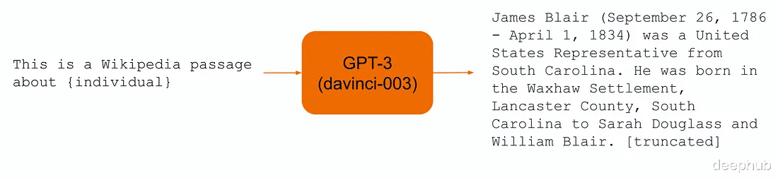
,这些生成的段落在句子层面上被手工标注为事实。每个句子被标记为主要不准确,次要不准确,或准确。总共有1908个句子被注释,大约40%的句子主要不准确,33%的句子次要不准确,27%的句子准确。
为了评估注释者的一致性,201个句子有双重注释。如果注释者同意,则使用该标签;否则选择最坏情况的标签。Cohen’s kappa测量的注释者间一致性在准确、次要不准确和主要不准确之间进行选择时为0.595,在次要/主要不准确合并到一个标签时为0.748。
评价指标AUC-PR是指准确率-召回率曲线下的面积,是用来评价分类模型的指标。
实时幻觉检测我们可以构建一个实时幻觉检测的Streamlit应用。如前所述,最好的度量是LLM自相似性得分。我们将使用0.5的阈值来决定是显示生成的输出还是显示免责声明。
import streamlit as stimport utilsimport pandas as pd# Streamlit app layoutst.title('Anti-Hallucination Chatbot')# Text inputuser_input = st.text_input("Enter your text:")if user_input: prompt = user_input output, sampled_passages = utils.get_output_and_samples(prompt) # LLM score self_similarity_score = utils.llm_evaluate(output,sampled_passages) # Display the output st.write("**LLM output:**") if float(self_similarity_score) > 0.5: st.write(output) else: st.write("I'm sorry, but I don't have the specific information required to answer your question accurately. ")
我们看看结果。

聊天机器人的幻觉检测一直是人们讨论已久的质量问题。
我们只是概述的了目前的研究成果:通过生成对同一提示的多个响应并比较它们的一致性来完成。
还有更多的工作要做,但与其依赖于人工评估或手工制定的规则,让模型自己捕捉不一致似乎是一个很好的方向。
https://avoid.overfit.cn/post/f32f440c1b99458e86d3e48c70ddcf94
作者:Iulia Brezeanu
